
The previous post introduced the ray tracing project Manta Ray, which we put in motion by writing an image to the screen buffer of the renderer. Next, we’re going to take a look at vectors, rays and a simple camera system for the renderer.
Vectors
At the heart of ray tracers (or almost any graphical program for that matter) lay vectors. As you might already know, a vector is a quantity that has a magnitude and a direction, commonly represented by a line segment. We’ll be using vectors to denote many types of data within the program such as directions, locations, offsets and even colors.
Luckily, the base template we’re using has already implemented vector constructions and accompanying mathematics for us. Since we work in 3D space, the predefined float3 struct is just what we need; it stores x, y and z coordinate components with floating point precision and it has all the vector functions we’d need for now. Going forward, I will assume that you have a basic understanding of vector related mathematics!
New to vectors or do you need a refresher? This video is a great recap of everything you’d need to know about vector math!
Color simplification
At the moment we pass the screen->Plot function a uint for a color. Shifting bits around whenever we need to work with colors isn’t very intuitive, so let’s practice what we preach and use float3 to represent colors instead.
First, we define a color alias for float3:
1
2
// type alias for float3, defined below its existing struct implementation
using color = float3;
Let’s create a utility function that helps us convert a color back to a uint:
1
2
3
4
5
6
7
8
9
10
11
#pragma once

inline uint convert_color(const color& pixel_color)
{
    // convert the calculated values from a [0, 1] range to a [0, 255] RGB range,
    // then shift the bits to combine the colors in one unsigned integer
    return
        (static_cast<int>(255.0f * pixel_color.x) << 16) +
        (static_cast<int>(255.0f * pixel_color.y) << 8) +
        (static_cast<int>(255.0f * pixel_color.z));
}
Now we can reflect these changes in our main source file:
1
2
3
4
5
6
7
8
9
10
11
12
13
14
15
16
// this method is called once per frame while the application is running
void mantaray::Tick(float deltaTime)
{
    // clear the previously drawn frame by resetting the screen buffer to black
    screen->Clear(0);

    // loop over all the screen buffer pixels as if reading a book: left->right, top->bottom
    for (int y = 0; y < SCRHEIGHT; y++) for (int x = 0; x < SCRWIDTH; x++)
    {
        // calculate some values for the red, green and blue components of a pixel
        color pixel_color(float(x) / (SCRWIDTH - 1), 0.25f, float(y) / (SCRHEIGHT - 1));

        // draw the color to the current screen buffer pixel
        screen->Plot(x, y, convert_color(pixel_color));
    }
}
Ray tracing in a nutshell
In the previous post I mentioned that ray tracers try to simulate real-life physics. The image below gives an overview of a typical ray tracing scene:
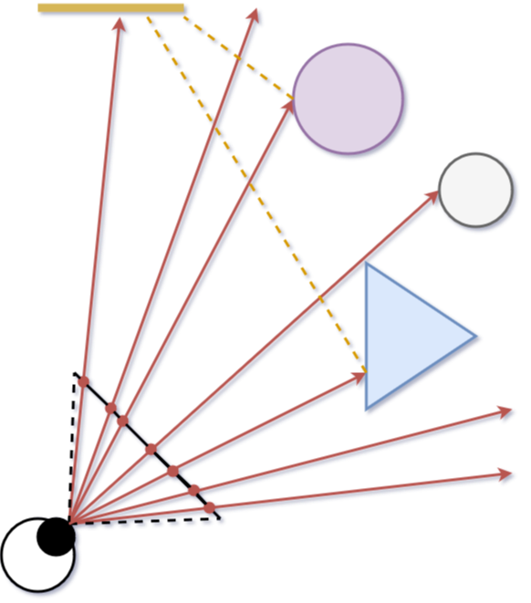 A simplified overview of a typical ray tracing scenario.
Here we see a camera (depicted as an eye) shooting rays into the scene through a virtual viewport (the black line). This is the core concept of ray tracing: sending rays through pixels, then computing the color seen along those rays to render an image. We can dissect this process into the following steps:
- Ray calculation: calculate the rays from the camera to every pixel on the virtual viewport (the red arrows). These rays are also called primary rays.
- Ray intersection: calculate the nearest intersection point between each ray and any object in the scene, if it exists. Only the nearest intersection is important; any intersection further along the ray is obstructed by the first one anyway!
- Ray color: compute a color for the found intersection points, summing up the contribution of any light sources visible from each point. This is achieved by so-called shadow rays (the yellow dashed lines).
For now, let’s solely focus on the first step. To calculate rays spawning from the camera, we’d need to (obviously) put both in the code somehow, which will be our next focus point.
You might have noticed that ray tracing handles light transport backwards; that is, from camera to light source. This gives the renderer a performance boost as we only care about the rays that’ll actually hit the camera.
Implementing rays
All ray tracers have some implementation in place to compute ray-specific values in order to render an image (I know, total shocker right?). A ray can be defined as an infinite half-line; basically a line in 3D space with a starting point. This leads to the following function:
\[P(t) = O + t\overrightarrow{D}\]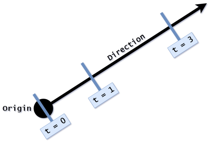 Where $O$ is the ray origin and $\overrightarrow{D}$ the (normalized) direction of the ray. Any 3D point $P$ along the ray can be found by plugging in values for $t$, where $t \geq 0$. In other words, different values for $t$ moves point $P$ along the ray. This will be useful to find the exact intersection points of a ray with objects in a scene.
Let’s add a ray class to the project which implements this functionality:
1
2
3
4
5
6
7
8
9
10
11
12
13
14
15
16
17
18
19
20
21
#pragma once

class ray
{
private:
    float3 m_origin;
    float3 m_direction;

public:
    // constructors, ray direction is normalized
    ray() {}
    ray(const float3& origin, const float3& direction)
        : m_origin(origin), m_direction(normalize(direction)) {}

    // getters
    float3 origin() const { return m_origin; }
    float3 direction() const { return m_direction; }

    // gets the position for the given t value
    float3 point(float t) const { return m_origin + t * m_direction; }
};
Normalizing the ray direction isn’t strictly necessary at this stage. However, forgetting to normalize when it does matter can lead to strange bugs. Be wary of this if you choose to omit it for now!
Implementing a camera
Next, the camera. The camera consist of a position and a virtual viewport; the viewport is comparable to a lens in a real camera.
To start, let’s define an aspect ratio for the screen buffer of the renderer (16:9 is a common standard), which we can use to set the screen resolution as well:
1
2
3
4
5
6
7
constexpr float m_aspect = 16.0f / 9.0f;
constexpr int m_scr_width = 640;
constexpr int m_scr_height = m_scr_width / m_aspect;

#define ASPECT      m_aspect
#define SCRWIDTH    m_scr_width
#define SCRHEIGHT   m_scr_height
For the viewport we will use the same aspect ratio to ensure the pixels are perfect squares. We could always change this later to get cool effects such as barrel- or pincushion distortion… Kinda like changing lenses on a camera!
The viewport will be two units in height, as will be the distance between the camera origin and the viewport (the focal length of a camera). To keep things simple, let’s put the camera origin at $(0, 0, 0)$. Recall from the previous post that the coordinate system in graphics applications starts in the top-left corner, where x and y are positive when going to the right and down respectively. Hence why I have chosen to do the same for the camera coordinate system, making the program less confusing. To respect the right handed coordinate system, the z-axis will be positive going into the screen; or differently phrased, the value of z will be larger when the depth is greater.
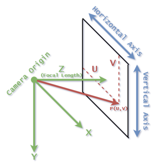 An overview of the camera and viewport geometry.
The last thing we need to set up is a way to position a ray relative to the viewport. By traversing the screen from the top-left corner, we can reach any pixel on the viewport by “walking” a certain distance along the horizontal and vertical axis vectors of the viewport. We denote this distance as $u$ for the horizontal axis, and $v$ for the vertical one. This gives the following formula for any point on the virtual viewport:
\[P(u, v) = P_{topleft} + u\overrightarrow{D}_{hor} + v\overrightarrow{D}_{vert}\]Where $u, v \in [0, 1]$. Thus, $u$ and $v$ determine the ratio, where $(u, v = 0)$ is the top-left corner, and $(u, v = 1)$ the bottom-right one (similar to the color rendering in the previous post!).
Now that we finally have a position on the virtual viewport, we can construct a ray from the camera through this position by subtracting the camera origin:
\[\overrightarrow{D}_{ray} = P(u, v) - P_{origin}\]Pfew, time to translate this all to code:
1
2
3
4
5
6
7
8
9
10
11
12
13
14
15
16
17
18
19
20
21
22
23
24
25
26
27
28
29
30
31
32
33
34
35
36
37
#pragma once

class camera
{
private:
    float3 m_origin;
    float3 m_horizontal;
    float3 m_vertical;
    float3 m_focal;
    float3 m_upper_left_corner;

public:
    camera()
    {
        // initialize the viewport dimensions
        float viewport_height = 2.0f;
        float viewport_width = ASPECT * viewport_height;
        float focal_length = 2.0f;

        // create the viewport by defining the horizontal/vertical/focal vectors
        // and set the camera origin at (0.0f,0.0f,0.0f)
        m_origin = float3(0.0f);
        m_horizontal = float3(viewport_width, 0.0f, 0.0f);
        m_vertical = float3(0.0f, viewport_height, 0.0f);
        m_focal = float3(0.0f, 0.0f, focal_length);

        // calculate the position of the upper left corner of the virtual viewplane,
        // using the created vectors/positions
        m_upper_left_corner = m_origin - m_horizontal / 2.0f - m_vertical / 2.0f + m_focal;
    }

    // fire a new ray from the camera, with u and v defining the ratio to the viewport
    ray fire_ray(float u, float v) const
    {
        return ray(m_origin, m_upper_left_corner + u * m_horizontal + v * m_vertical - m_origin);
    }
};
To test the new camera, I implemented a simple temporary function which returns a color for a ray depending on its y direction called ray_color. All these changes are reflected in the main source file as follows:
1
2
3
4
5
6
7
8
9
10
11
12
13
14
15
16
17
18
19
20
21
22
23
24
25
26
27
28
29
30
camera cam;

// returns a background gradient depending on the y direction of a primary ray
color ray_color(const ray& r)
{
    // convert a ray's y value from roughly [-0.5, 0.5] space (due to vector normalization) to [0, 1] space
    float t = r.direction().y + 0.5f;

    // linear interpolation of the background, t = 0 gives blue-ish, t = 1 gives white, blend in-between
    return lerp(color(0.5f, 0.7f, 1.0f), color(1.0f), t);
}

// this method is called once per frame while the application is running
void mantaray::Tick(float deltaTime)
{
    // clear the previously drawn frame by resetting the screen buffer to black
    screen->Clear(0);

    // loop over all the screen buffer pixels as if reading a book: left->right, top->bottom
    for (int y = 0; y < SCRHEIGHT; y++) for (int x = 0; x < SCRWIDTH; x++)
    {
        // calculate the u and v value for the current pixel and fire a ray using these values
        float u = float(x) / (SCRWIDTH - 1);
        float v = float(y) / (SCRHEIGHT - 1);
        color pixel_color = ray_color(cam.fire_ray(u, v));

        // draw the color to the current screen buffer pixel
        screen->Plot(x, y, convert_color(pixel_color));
    }
}
Behold! Our first “ray traced” image:
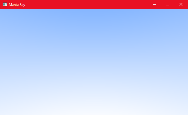 Mr. Blue Sky, please tell us why, you had to hide away for so long (so long)!
It’s… Rather dull for the amount of effort. However! We made some major strides coming to this point. The backbone of our renderer is now (mostly) in place. Next time we will implement step 2 of the rendering process: ray intersection! See ya later. 🐊